路网匹配-备忘录

路网匹配研究综述

轨迹模式挖掘具体是指什么呢？

共同移动模式：多个目标连续k个时间戳共同移动
轨迹聚类：

关心的问题

路网匹配算法所能解决的数据特点：采样频率。

如何判断路网匹配算法的实际效果

几何匹配算法

点到点的匹配

点到线的匹配

线到线的匹配

路网地图下载

开源工具

Github Osmxn，通过如下命令启动环境，本地文件夹/home/jingtao/repos/osm/osmnx，访问对应的8888端口进入jupyter lab。

1	docker run -itd -p 8888:8888 -v "$PWD":/home/jovyan/work gboeing/osmnx:latest

下载对应区域的代码如下，更多下载方式参考Osmxn Example。

# 下载并保存路网信息
import osmnx as ox
import time
from shapely.geometry import Polygon
import os

def save_graph_shapefile_directional(G, filepath=None, encoding="utf-8"):
    # default filepath if none was provided
    if filepath is None:
        filepath = os.path.join(ox.settings.data_folder, "graph_shapefile")

    # if save folder does not already exist, create it (shapefiles
    # get saved as set of files)
    if not filepath == "" and not os.path.exists(filepath):
        os.makedirs(filepath)
    filepath_nodes = os.path.join(filepath, "nodes.shp")
    filepath_edges = os.path.join(filepath, "edges.shp")

    # convert undirected graph to gdfs and stringify non-numeric columns
    gdf_nodes, gdf_edges = ox.utils_graph.graph_to_gdfs(G)
    gdf_nodes = ox.io._stringify_nonnumeric_cols(gdf_nodes)
    gdf_edges = ox.io._stringify_nonnumeric_cols(gdf_edges)
    # We need an unique ID for each edge 和 fmm给出的代码有区别，注意更改
    gdf_edges=gdf_edges.reset_index()
    gdf_edges["fid"] = gdf_edges.index
    # save the nodes and edges as separate ESRI shapefiles
    gdf_nodes.to_file(filepath_nodes, encoding=encoding)
    gdf_edges.to_file(filepath_edges, encoding=encoding)

print("osmnx version",ox.__version__)

place ="Beijing, China"
G = ox.graph_from_place(place, network_type='drive', which_result=2)
save_graph_shapefile_directional(G, filepath='beijing')

无脑执行上述代码，就能获取北京市的行车路网图，由于北京市路网数据量庞大，执行时间会比较久。

路网匹配工具

FMM

Github地址

预处理：

Upper Bounded Origin Destination Table（计算所有顶点对之间的最短路经，且最短路径长度不能超过一个阈值）

路网匹配：

候选项搜索 CS
- candidate search
- 在点p的r半径范围内搜索k个最近的候选路段，组成每个轨迹点的候选边集合C
最佳路径匹配 OPI
- optimal path inference
- 转移概率(transition)tp，
  - 定义两种距离，
    一个是两个轨迹点之间的距离为$d_{n, n+1}$，
    另一个是这两个轨迹点所匹配到的候选边之间的最短路径距，记为$l_{n, n+1}^{C}$，具体计算方法如下 \[ l_{n, n+1}^{C}=\left\{\begin{array}{lc} C_{n+1} \cdot \lambda-C_{n} \cdot \lambda, & \text { if } C_{n} \cdot e=C_{n+1} \cdot e, C_{n} \cdot \lambda \leq C_{n+1} \cdot \lambda \\ C_{n} \cdot e . L-C_{n} \cdot \lambda+l_{n, n+1}^{N}+C_{n+1} \cdot \lambda, & \text { else } \end{array}\right. \]
  - 状态转移公式最终定义为 \[ t p\left(C_{n}, C_{n+1}\right)=\frac{\min \left(d_{n, n+1}, l_{n, n+1}^{C}\right)}{\max \left(d_{n, n+1}, l_{n, n+1}^{C}\right)} \]
- 发射概率(emission)ep，候选边到轨迹点的距离的高斯分布之后的结果
- HMM发挥作用于此
- 经过在每个轨迹点（观测点）的候选边中选择到的的最优边，获取到O_path
完成路径构造 CPC
- complete path construction，在O_path中边不相接的地方，根据UBODT预计算的最短路径直接补全。
- 输出边的序列为C_path
地理路径构造
- 有了C_path之后，根据边的地理曲线，得到最终的结果

长距离路由查询

在UBODT中只存储了距离有限的顶点对之间的距离，若要查询的顶点之间的距离在UBODT中不存在，则可以采用直接调用dijkstra算法进行计算，或者返回UBODT中的最大距离阈值，或者直接剪枝（根据观测到的轨迹顶点之间的距离来判断）。论文中具体给出了四种模型的解决方案。

对反向移动的惩罚

反向移动出现的两个原因：

GPS坐标偏差比较大，造成反向移动的路径的概率十分的高
在最佳的路径匹配的过程中，出现了其中的一条反向运动边

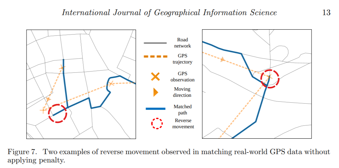
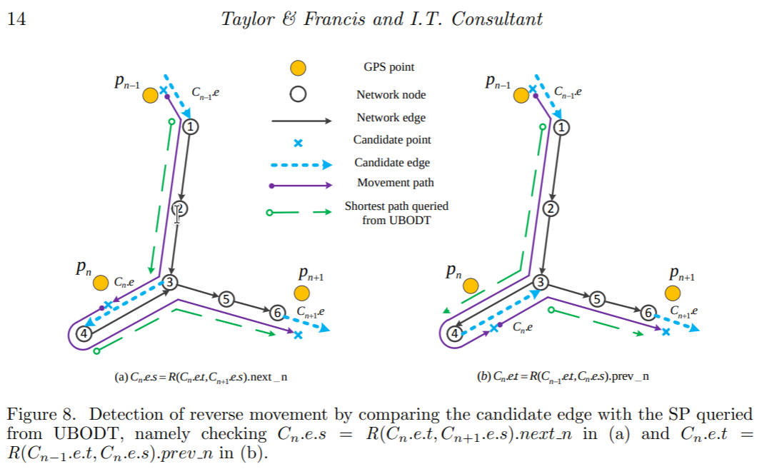
论文中提出的解决办法是，对这种相接之后会出现反向边的情况，添加惩罚（添加到SP中），提高被选中的门槛，其中pf是惩罚因子 \[ \tilde{l}_{n, n+1}^{C}=\left\{\begin{array}{ll} l_{n, n+1}^{C}+p f * C_{n} \cdot L & \text { if record.next\_n }=C_{n} . e . s \\ l_{n, n+1}^{C}+p f * C_{n+1} \cdot L & \text { else if record.prev\_n }=C_{n+1} . \text { e.t } \\ l_{n, n+1}^{C} & \text { else. } \end{array}\right. \]

评价方法

对算法的效率进行了评估

对算法的准确性进行了评估，ground truth是人工标注的

对算法对抗反向路径进行了评估

WRY